
Training regimes, regularization schemes, and architecture enhancements are crucial for effective deep learning. We shall name them “Dark Magic Tricks”. In this article, we review useful dark magic tricks, accompanied by examples and use-cases. We also compile a generic “checklist” of tricks testing, that can be used to upgrade any existing deep learning repository.
Dark magic tricks are usually not fully supported by deep mathematical background but are more empirically and heuristically based. Due to that, in many cases they are overlooked and briefly mention as implementations details in academic articles, sometimes even visible only by inspecting source codes.
The lack of fundamental understanding and the heuristic nature of these tricks, in addition to their importance and effectiveness, is the reason we named them “Dark Magic”.
Despite the relative disregarding, we argue that the difference between mediocre and top repositories is almost always due to better dark magic tricks. Even for articles that claim to reach new SotA scores using a unique novelty, in almost all cases the novelty is accompanied by very effective usage of existing dark magic tricks.
There is no trick that always works, and has “correct” hyper-parameter values. You usually need to choose the relevant tricks for each problem and tune their hyper-parameters. However, knowing and understanding common best practices can increase dramatically the chance to use dark magic tricks effectively and get top scores.
We have compiled a generic checklist of dark magic tricks and best practices, that we try and test each time we start a new repository or upgrade an existing one. For each checklist trick, we always try to recommend a specific default option, instead of suggesting a long list of possibilities. Each recommendation is accompanied by example and uses cases that were thoroughly tested and reviewed. While our main focus was on classification datasets, we believe that our checklist has a good chance to generalize to other tasks and datasets.
Tricks Testing Checklist
Training Schemes:
- Which learning rate regime to choose
- Which optimizer to choose
- Should we always pretrain a model on ImageNet
- Which batch size to use (-)
Regularization Tricks:
- AutoAugment
- Weight decay
- Label smoothing
- Scheduled regularizations
- Mixup
- Auxiliary loss (-)
- Crop factor, padding and resizing schemes(-)
- Drop path (-)
- CutOut (-)
Architecture Enhancements:
- Squeeze-And-Excite (SE) layers
- Stem activation functions
- Attention pooling (-)
While we, of course, can’t cover all the existing dark magic tricks, we found the checklist above very useful and were able with it to improve our scores significantly on multiple datasets — CIFAR10, CIFAR100, ImageNet, Palitao-102K, Alicool, COCO keypoints, Market-1501, SVHN, Freiburg-grocery and more. In the following sections, we will dive in and analyze the different tricks on the checklist.
Due to space considerations, tricks marked with (-) are left for future posts.
Training Schemes
Which Learning Rate Regime to Choose
We experimented a lot with different kinds of learning rate regimes, including gamma decay, cosine annealing, heuristics (“reduce learning rate by factor 0.1 in epochs 50 and 75…”) and more.
We found that the learning rate regime which is the easiest to tune and generalize best to multiple datasets is “Cosine power annealing”, that can be seen as an average between cosine annealing and gamma decay via a control parameter P:

P permits tuning of the curves decay rate such that it maintains a high learning rate for the first few epochs, while simultaneously taking a shallower slope during the final third of epochs. We usually choose P=2 or P=4.
We also found that given a fixed number of epochs, repeated cycles of cosine power annealing with decaying amplitude gave us better test scores than a single cycle. Another advantage of repeated cycles is that during the training we get improving estimations for the final accuracy.
Finally, we found that a small warm-up duration stabilizes our training and enable us to use a larger initial learning rate, which accelerates the convergence.
To conclude, the learning regime we found that works best on multiple datasets is cycles of cosine power annealing, with decaying amplitude and initial warm-up, as presented in the following graph:
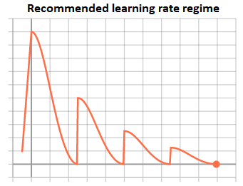
Comparing cycles of power cosine against simple gamma decay and cosine annealing will sum up to 3 trials.
Which Optimizer to Choose
Currently, most top deep learning repositories are using simple SGD with momentum optimizer, instead of fancier optimizers like ADAM or RMSProp, mainly because SGD uses less GPU memory and has significantly lower computational cost.
For multiple datasets, we found that SGD with Nesterov-momentum outperforms plain SGD with momentum optimizer while having the same GPU memory consumption and a negligible additional computational cost. An example from ImageNet testings:

Hence we recommend using SGD with Nesterov momentum optimizer as the default option for deep learning training. Comparing Nesterov momentum to regular SGD with momentum and ADAM optimizers will sum up to 3 trials.
Should We Always Pretrain a Model on ImageNet
A widespread practice for computer vision deep learning is to pretrain a model on ImageNet.
While this approach showed great success in the past, it was usually used on large models like ResNet or Inception, that contain tens of millions of parameters.
Nowadays, there are many models with comparable performances to ResNet, but with an order of magnitude fewer parameters, such as MobileNet, ShuffleNet, and XNAS.
We found that when training these smaller models on different datasets, pretraining on ImageNet may hurt the performance significantly, as this example on COCO keypoint detection dataset shows:
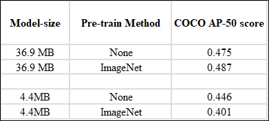
Hence our recommendation is to consider carefully the effectiveness of pretraining a model on ImageNet, especially for small models.
Comparing training without and with ImageNet pretraining will sum up to 2 trials.
Regularization Tricks
AutoAugment
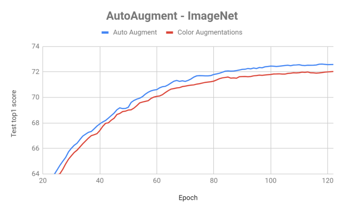
AutoAugment is a seminal work where learned augmentations replaced standard color augmentations. Three AutoAugment policies were learned, for the datasets: CIFAR10, ImageNet and SVHN.
When using these policies, we were able quickly to reproduce the article results and get an improvement over standard color augmentations

However, what about other datasets, where no specific policy of AutoAugment was learned?
We advise against trying to learn dedicated augmentations regimes for your dataset since it requires a substantial amount of GPU hours and extensive tuning of hyper-parameters, which can take weeks over weeks. Notice that newer works that claim to learn augmentation policies faster studied exactly the same datasets as the original AutoAugment article.
Instead of trying to learn a tailor-made augmentation regime for your datasets, we suggest using existing AutoAugment policies. Here are results we got for Freiburg-groceries and Alibaba-internal Palitao-102K datasets:
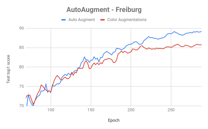
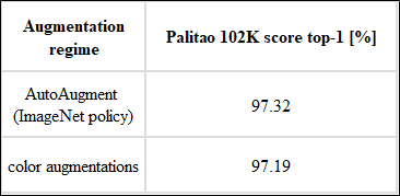
Hence we recommend trying using AutoAugment existing policies instead of plain color augmentation.
Comparing AutoAugment (preferable ImageNet policy) to standard color augmentations will sum up to 2 trials.
Weight Decay
While mentioned in every beginner’s deep learning course, weight decay does not receive the attention it deserves among regularization techniques. Most repositories don’t seem to invest lots of effort in optimizing the weight decay, and just use a generic value, usually 5e-5 or 1e-5.
We argue that weight decay is one of the most influential and important regularization techniques. Adjusting the weight decay is crucial for obtaining top scores, and the wrong value of weight decay can be a major “blocker”.
For example, here are tests we did to optimize weight decay on ImageNet and CIFAR10:
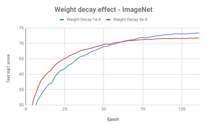

We can see that for both datasets optimizing the weight decay gave a significant boost to the test score.
Hence we recommend optimizing weight decay instead of using a generic value.
We suggest testing at least 3 values of weight decay, a “generic” value (~5e-5), bigger weight decay and a smaller one, summing up to 3 trials. If significant improvement is seen, do more tests.
Label Smoothing
Label smoothing is an important classification training trick that appears in most repositories, usually with a default smoothing value of 0.1, which people rarely change.
With label smoothing, we edit the target labels to be:
target = (1 — epsilon) * target + epsilon / (num_classes-1).
We found that label smoothing improves the training score for almost any classification problem, where for datasets with large number of labels like Palitao-102K, larger values of label-smooth (>0.1) gave further improvement:
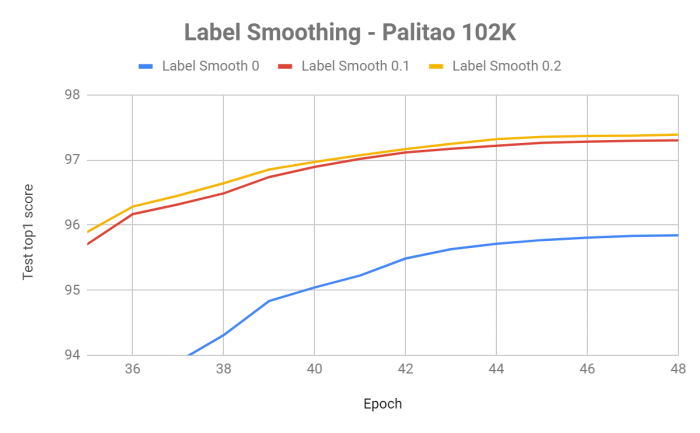

Hence we recommend using label smoothing for classification problems. This is especially important for datasets with a large number of labels.
We recommend doing checklist trials for 3 values of label smoothing: 0, 0.1, and 0.2.
Scheduled Regularizations
It is a very common practice to govern a regularization technique by one (or more) fixed hyper-parameter values. However, for learning-rate it is clearly absurd to think that a fixed value is the optimum solution, and people always use a scheduling regime, usually decreasing the learning rate during the training. Why shouldn’t we use similar scheduling regimes for regularization techniques?
An interesting question would be: should we increase or decrease regularization “power” during the training? Here is where we stand — overfitting happens toward the end of the training, when the learning rate is low and the model has almost fully converged. Hence we argue that we need to increase regularization strength as the training progresses, and prevent the overfitting at the final training stages.
Here is an example: we tested different values of weight decay on CIFAR100 dataset, and found very clearly that 3e-4 is the optimum value (for a fixed weight decay).
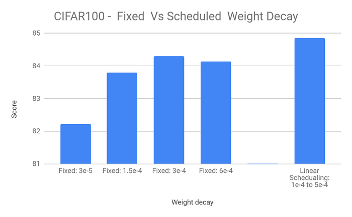
A simple test with scheduled weight decay, where we linearly increase its value during the training, immediately gave improvement over the best fixed-value option:
We are still researching other scheduling schemes — for example, instead of changing a regularization factor linearly (linear policy), we can increase it after each learning cycle (cycles policy), or make it proportional to the learning rate (learning rate policy):
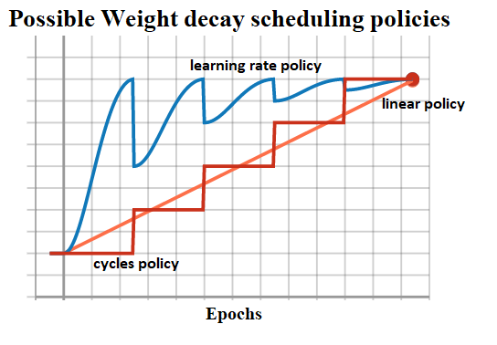
For now, we recommend that once you established an optimal value for (fixed) weight decay, compare it against linear scheduled weight decay regime, summing up to 2 trials.
Mixup
Mixup technique was suggested in Facebook article “mixup: Beyond empirical risk minimization” and gained some popularity since. We followed the article implementation of mixup:


